I like to automate things whenever possible and filling out forms that must be filled out over and over is one thing I like to make easier if at all possible.  Unfortunately Excel doesn’t have anything built in to take a day number and apply the appropriate suffix on it, as seen in the picture above.  You can easily write a formula to do it for you and this is how…

How to Write a Formula to Append the st, nd, or rd to the End of a Date Number in Microsoft Excel–Example: 6th Day of Feb

Step 1: Analyze what numbers need what.

Thankfully there are only 3 options and this is all the ways a day can pan out:  1st, 2nd, 3rd, 4th, 5th, 6th, 7th, 8th, 9th, 10th, 11th, 12th, 13th, 14th, 15th, 16th, 17th, 18th, 19th, 20th, 21st, 22nd, 23rd, 24th, 25th, 26th, 27th, 28th, 29th, 30th, and 31st.  The way it turns out, all of the numbers end in “th” except for seven of them: 1, 2, 3, 21, 22, 23, and 31.  If we break down the non-“th” numbers they categorize like this:

st: 1, 21, 31
nd: 2, 22
rd: 3, 23

This gives us four total categories, which we can handle with “nested if” statements in Excel.

Step 2: Sketch out your formula.

The basics of it will be like this:

If Day = (1 OR 21 OR 31) then Append “st”
If Day = (2 OR 22) then Append “nd”
If Day = (3 OR 23) then Append “rd”
Else Append “th”

Step 3: Write the formula.

The way Excel “IF” statements are laid out is as follows:

IF(logical_test,value_if_true,value_if_false)

We have more than 1 possible true values so we need to account for that.  The easiest way is through the use of Excel’s “OR” function.  It performs in the following way:

OR(logical1,logical2,…)

BTW: the way to “append” text to other text is though the use of an “&” symbol.  If you put A2&”st” it will append an “st” to whatever is in the cell A2.

If “A1” contains the date you are wanting to perform this function on then this is how you would write the formula:

=IF(A1=””,””,DAY(A1)&IF(OR(DAY(A1)=1,DAY(A1)=21,DAY(A1)=31),”st”,IF(OR(DAY(A1)=2,DAY(A1)=22),”nd”,IF(OR(DAY(A1)=3,DAY(A1)=23),”rd”,”th”))))

Note: I put in first A1=”” logical test so the formula result in a blank (“”) if there is no date in cell A1, otherwise you’ll get the “ELSE” result appended to a blank.  Hopefully this helps you out.One way I’ve implemented this is to have the date entered in a cell outside the print area of a waiver form, as seen below:

Implementation of formula

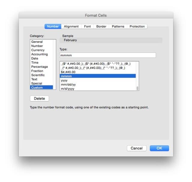
Note: To get only the Month to show up in a cell simply place an equals sign in the cell and then the cell name of the date.  Then format the cell as follows: From the menu at the top of the screen select Format > Cell (or Command-1 on a Mac).  Pick “Custom” in the left column and type “mmmm” in the Type: box as seen below:

Formatting Cells for Month name only

To get the year only point the cell to the date like described below and type “yyyy” in the Type: box.

Note: This is also referred to as “Adding Ordinal Notation to Dates” but I’m not that sophisticated (couldn’t even spell it close enough the first time for autocorrect to help me spell sophisticated either).